Resampling Asset Prices the Right Way

New monograph from Richard Crump and Nikolay Gospodinov that I think deserves more attention: Resampling Asset Prices: An Identity-Based Approach (Cambridge Elements in Quantitative Finance, 2026). Available free here, with a full MATLAB replication package on GitHub.

The core idea

Figure 3: Nonparametric vs parametric bootstrap of the Cochrane-Piazzesi tent shape — The nonparametric identity-based bootstrap (top) reproduces the Cochrane-Piazzesi "tent shape" in bond return regressions. The standard parametric VAR(1) bootstrap (bottom) completely misses it. Black line = sample estimate, colored lines = individual bootstrap draws.

The idea is simple and pretty neat. When you bootstrap bond yields or the dividend-price ratio directly, you’re resampling objects with massive persistence and cross-sectional dependence. That makes it hard to do well — the bootstrap works much better with independent things.

So instead: bootstrap primitive objects that are approximately i.i.d. (difference returns for bonds, price growth and dividend growth for equities), then rebuild everything you actually care about — yields, returns, the d/p ratio — through accounting identities. This is a really nice intersection between statistics and many of the important accounting identities in finance.

The equity case

Figure 7: Main components of equity returns — returns, price growth, dividend growth, and the dividend-price ratio — The primitive objects for the equity bootstrap: gross returns and price growth (top row) are roughly i.i.d. Dividend growth (bottom left) has pronounced seasonality. The dividend-price ratio (bottom right) is highly persistent. S&P 500, 1952–2023.

For equities, the key identity is just the definition of a stock return:

Return = Price Growth + Dividend Growth × Lagged Dividend-Price Ratio

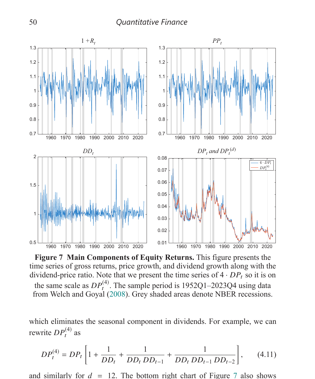
Or in their notation: $1 + R_t = PP_t + DD_t \cdot DP_{t-1}$, where $PP_t = P_t/P_{t-1}$ is price growth, $DD_t = D_t/D_{t-1}$ is dividend growth, and $DP_t = D_t/P_t$ is the dividend-price ratio. This always holds — it’s accounting, not a model.

In logs, the dividend-price ratio satisfies a recursive identity:

\[dp_t = dp_{t-1} + dd_t - pp_t\]

The correlation between returns and changes in d/p is about −0.98 in the data, and that’s mechanical — it comes from the identity. If you bootstrap returns and the d/p ratio separately, which is what standard resampling does, you break this link. Your resampled data are internally inconsistent. And when you run predictive regressions on inconsistent data, your inference is wrong.

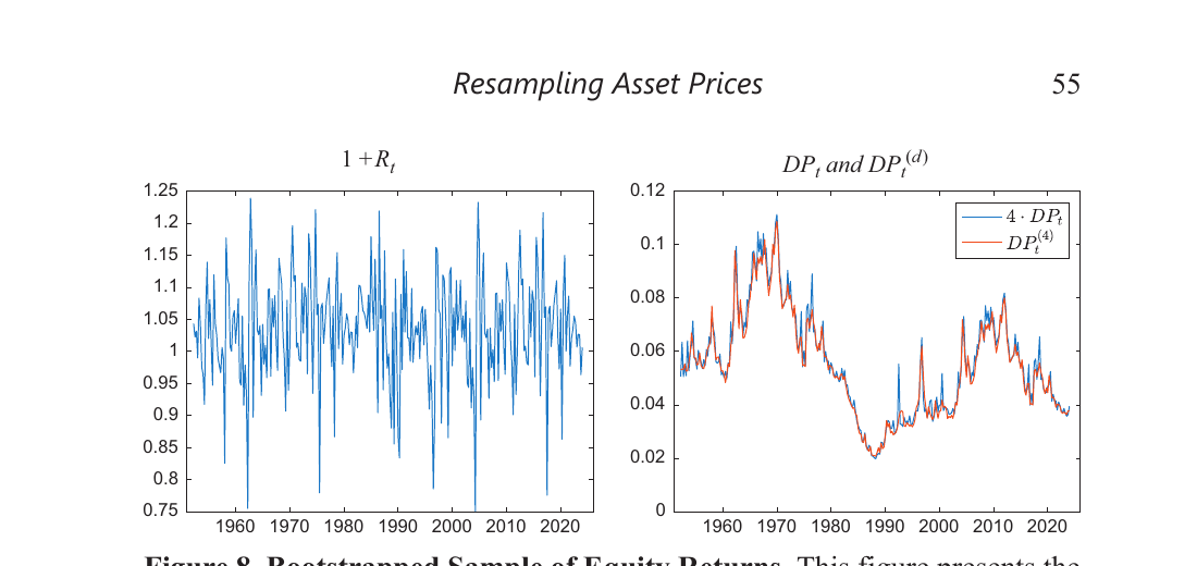
Crump and Gospodinov’s fix: bootstrap the primitives — price growth and dividend growth, which are roughly i.i.d. and easy to resample. Then rebuild the d/p ratio and returns through the identity. The high persistence of d/p — which makes direct bootstrapping so hard — emerges naturally from accumulating many small $dd_t - pp_t$ terms. No parametric model needed. [-1-] [-1-] They also build in a seasonal block bootstrap that handles the quarterly dividend payment pattern, which is a nice practical touch. Dividends have pronounced seasonality that would mess up a naive bootstrap.

Figure 8: A single bootstrap draw of equity returns and the dividend-price ratio — A single bootstrap draw: bootstrapped returns (left) and the dividend-price ratio (right). The bootstrap resamples only price growth and dividend growth, but the reconstructed d/p ratio captures the same persistent dynamics as the real data.

The bond case

Same logic for bonds. Excess returns are partial sums of “difference returns” — the return from buying an $n$-maturity bond and shorting an $(n-1)$-maturity bond:

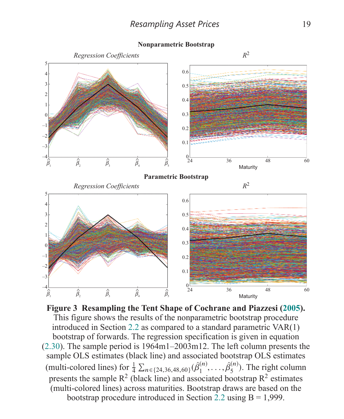
\[rx_t^{(n)} = \sum_{i=2}^{n} dr_t^{(i)}\]

Difference returns are well-behaved (roughly i.i.d.) because the cross-sectional differencing strips out the persistence that makes yields and forwards so hard to work with. The full yield curve can be rebuilt from difference returns plus an initial condition via identities. So bootstrap the difference returns, reconstruct everything else.

The key insight in both cases: the bootstrap never touches the persistent objects directly. It resamples things that are easy to resample, and the persistence, cross-sectional dependence, and factor structure all come back for free through the accounting identities.

Three findings I need to incorporate into my own work

1. Newey-West standard errors are way too small

In their simulations, Newey-West rejects at 20–37% for a nominal 10% test. The Crump-Gospodinov identity-based bootstrap gets empirical size right at roughly 10%, with minimal power loss relative to an infeasible oracle benchmark. Even the improved HAR estimator from Lazarus et al. (2018) over-rejects at 13–30%.

If you’re doing predictive return regressions with HAC standard errors, this should worry you. [-2-] [-2-] As a Bayesian, this seems right to me – the amount of information in these highly persistent, overlapping series is much less than the sample size suggests, and frequentist standard errors don’t account for that.

2. Inflation doesn’t actually predict bond returns

Using the bootstrap, the p-values for inflation as a predictor of nominal excess bond returns are all above 0.43. Using Newey-West? All below 0.06. Same regression, same data — opposite conclusions.

The bootstrap properly internalizes the co-movement between yields and realized inflation in each resampled path, which standard approaches miss entirely. The paper argues that information about near-term inflation is already embedded in the yield-based predictors.

3. For equities, d/p predicts returns and not much else does

The dividend-price ratio is significant at p < 0.03 across frequencies and horizons. But once you condition on d/p, none of the 12 Welch-Goyal predictors add anything — including book-to-market, earnings-price ratio, default spreads, term spreads, T-bill rates, or inflation.

This is the in-sample version of what Welch and Goyal (2008) showed out of sample, but now with inference you can actually trust. The bootstrap respects the identity linking returns, prices, and dividends, so the ~−0.98 correlation between returns and d/p changes is preserved in every bootstrap draw. Standard methods don’t do this.

Bonus: PCA and the yield curve

There’s also a striking result on PCA and the yield curve that’s worth knowing about. The famous “3 factors explain 93%+ of yield curve variation” result is partially mechanical — it arises from the overlapping maturity structure of how we construct yields from forwards, not necessarily from a genuinely low-dimensional factor space.

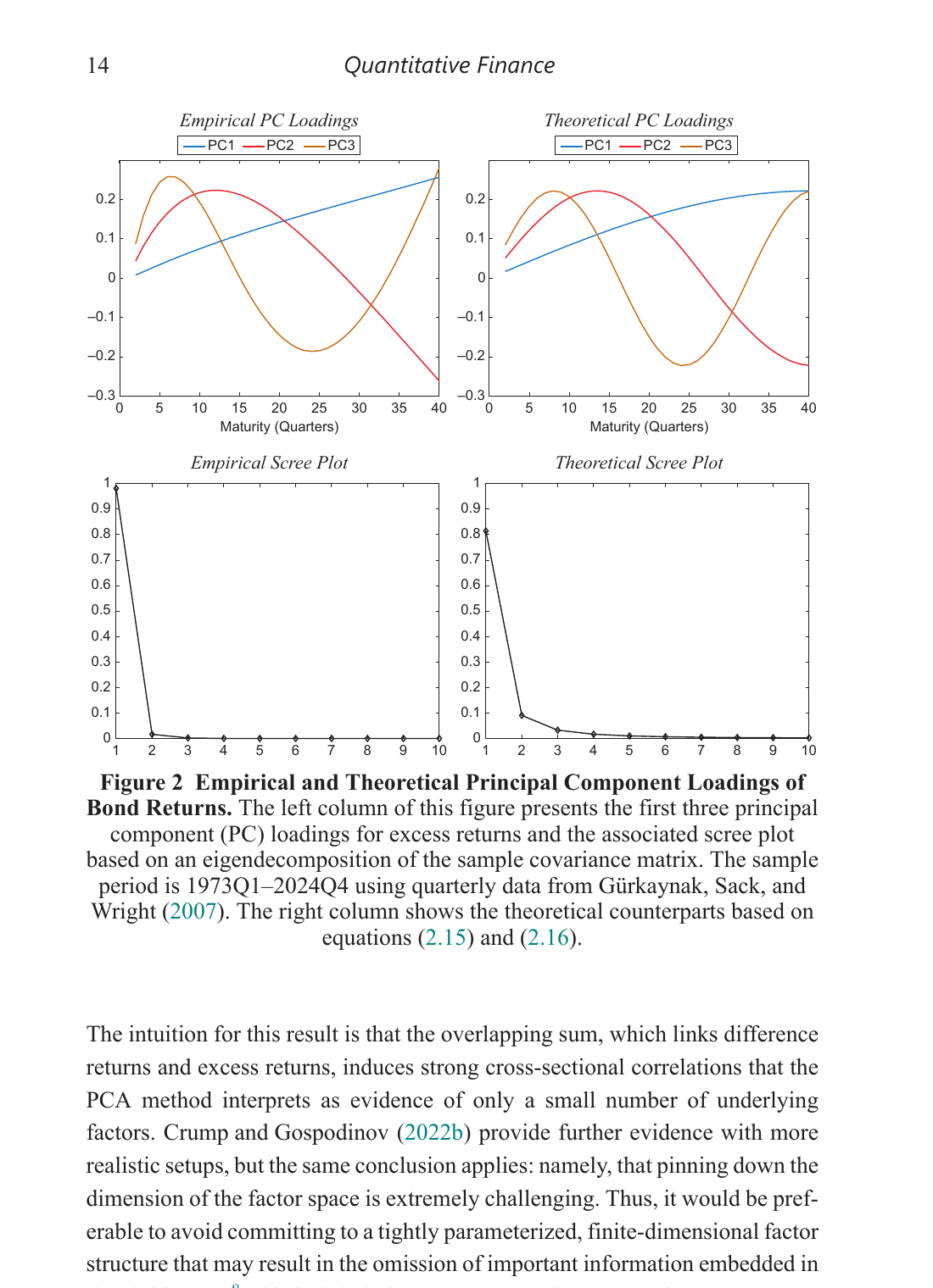
Figure 2: Empirical vs theoretical PCA loadings — the 3-factor structure is mechanical — Left column: empirical PCA loadings and scree plot from U.S. Treasury data (1973–2024). Right column: theoretical counterparts assuming N-1 independent factors. The "level, slope, curvature" pattern and the 3-factor dominance in the scree plot arise mechanically from the overlapping maturity structure.

Crump and Gospodinov show that even if difference returns were driven by $N-1$ independent factors (i.e. the covariance matrix of difference returns is proportional to the identity), PCA on excess returns would still show ~3 dominant components. The overlapping partial-sum structure ($rx^{(n)} = \sum dr^{(i)}$) induces the cross-sectional correlation that PCA interprets as a low-dimensional factor structure. The “level, slope, curvature” pattern in the loadings emerges mechanically. [-3-] [-3-] This result is from Crump and Gospodinov (2022, Econometrica). The implication for anyone building term structure models: committing to a 3-factor structure may omit important information.

This matters for anyone building factor models of the term structure — and it’s another argument for the nonparametric approach, which doesn’t take a stand on the number of factors.