Curated colour palettes for R • japanesecolors

149 curated colour palettes in four collections: Retro, Minimalism, Kawaii and Avant Garde.

Every palette is an exported character vector of hex colours, so the API is just the palette’s name.

Available for R and Python.

Installation

# install.packages("pak")
pak::pak("paulgp/japanesecolors")

# Python
pip install "japanesecolors[plot]"

Usage

library(japanesecolors)

kawaii_tri_07
#> [1] "#3D7EB4" "#DF4472" "#E68C5F"

Which means palettes work anywhere R takes colours:

barplot(c(6, 9, 4, 7), col = avantgarde_four_04, border = NA, axes = FALSE)

Bar chart of four bars coloured with the avantgarde_four_04 palette.

show_palette(minimalism_multi_02)

The seven swatches of minimalism_multi_02, each labelled with its hex value.

ggplot2

library(ggplot2)

ggplot(iris, aes(Sepal.Length, Sepal.Width, colour = Species)) +
  geom_point(size = 2.5) +
  scale_colour_japanesecolors("kawaii_tri_07") +
  theme_minimal()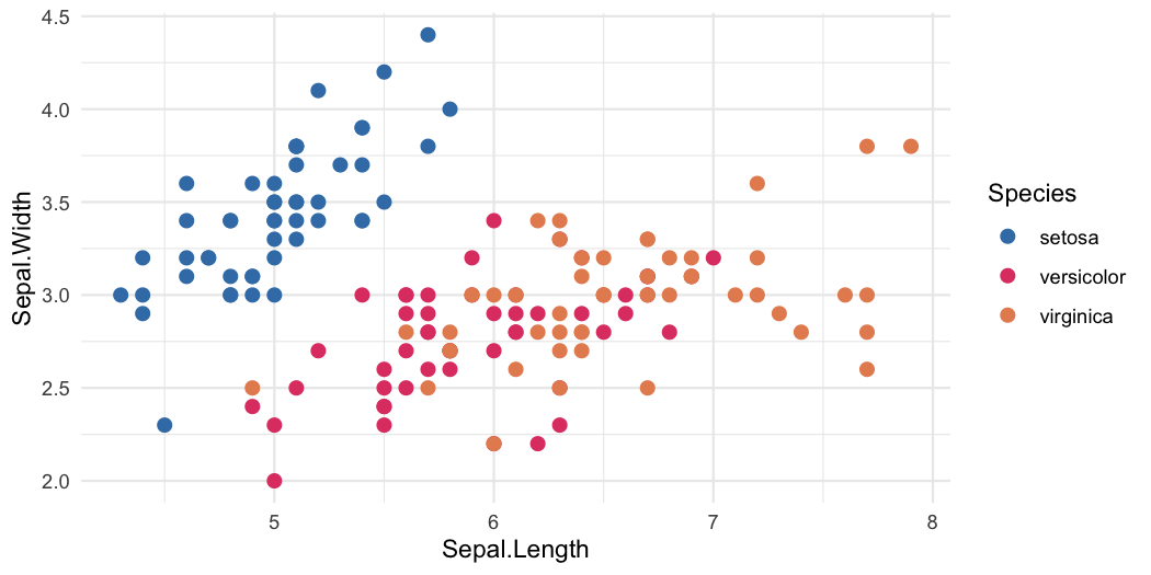

Scatter plot of iris sepal measurements, the three species coloured with kawaii_tri_07.

scale_fill_japanesecolors() and scale_color_japanesecolors() work the same way, or pass the vector straight to scale_colour_manual(values = kawaii_tri_07).

The collections

Collection	Palettes	Provisional
Retro	55	7
Minimalism	28	0
Kawaii	30	2
Avant Garde	36	4

Two example palettes from each of the four collections, shown as rows of colour swatches.

Browsing

IDs are <collection>_<type>_<nn>, where type is bi, tri, four or multi. They are stable API.

palettes("kawaii", type = "tricolor")[, c("id", "n_colors", "status")]
#>               id n_colors      status
#> 1  kawaii_tri_01        3 transcribed
#> 2  kawaii_tri_02        3 transcribed
#> 3  kawaii_tri_03        3 transcribed
#> 4  kawaii_tri_04        3 transcribed
#> 5  kawaii_tri_05        3 transcribed
#> 6  kawaii_tri_06        3 transcribed
#> 7  kawaii_tri_07        3 transcribed
#> 8  kawaii_tri_08        3 transcribed
#> 9  kawaii_tri_09        3 transcribed
#> 10 kawaii_tri_10        3 transcribed
#> 11 kawaii_tri_11        3 transcribed
#> 12 kawaii_tri_12        3 transcribed
#> 13 kawaii_tri_13        3 transcribed
#> 14 kawaii_tri_14        3 transcribed
#> 15 kawaii_tri_15        3 transcribed
#> 16 kawaii_tri_16        3 transcribed
#> 17 kawaii_tri_17        3 transcribed
#> 18 kawaii_tri_18        3 transcribed
#> 19 kawaii_tri_19        3      review

# find one big enough for seven groups
palette_names(n = 7)
#> [1] "minimalism_multi_02" "minimalism_multi_05" "minimalism_multi_06"
#> [4] "kawaii_multi_03"

# look up by ID when the palette is chosen at runtime
get_palette("minimalism_multi_02")
#> [1] "#E66A5F" "#EDC2B6" "#CBB493" "#9E809B" "#395642" "#BFE3E7" "#CEBD35"

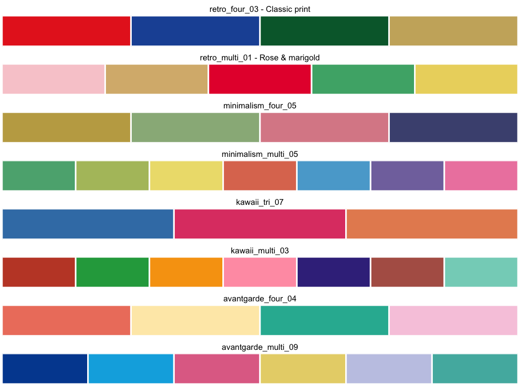
The visual gallery of all 149 palettes is on the package website.

Which ones work in a chart

These are design palettes, chosen to look good together rather than to encode categories, so most were never meant for data visualisation. 65 of the 149 screen well for it, on two criteria:

Colour-vision deficiency — colours that separate for a trichromat can collapse for a dichromat, so each palette is re-measured under simulated deuteranopia, protanopia and tritanopia.
Perceptual separation — categories have to read as different at a glance, in small marks.

Both use CIEDE2000 on a palette’s closest pair, since a palette is only as readable as the two colours most easily confused. A third check stops a near-white colour vanishing against the page.

palettes(dataviz_friendly = TRUE, n = 4)[, c("id", "min_delta_e", "min_delta_e_cvd")]
#>                   id min_delta_e min_delta_e_cvd
#> 1      retro_four_02        22.6            11.4
#> 2      retro_four_04        26.8            13.2
#> 3      retro_four_06        24.0            12.1
#> 4      retro_four_07        24.9            15.4
#> 5      retro_four_11        23.4            10.1
#> 6 minimalism_four_06        25.0            11.4
#> 7     kawaii_four_01        30.8            10.3
#> 8 avantgarde_four_01        33.9            13.2
#> 9 avantgarde_four_02        46.0            27.4

The measurements ship with every palette, so you can set your own bar. The thresholds are calibrated so that the Okabe-Ito palette, designed for colour-vision deficiency, passes — and palettes that separate well in normal vision but collapse for a dichromat, like ggplot2’s default hue scale, do not.

Worth knowing: no palette of five or more colours clears the bar. Keeping 5–8 colours mutually distinguishable under dichromacy is hard, and these palettes were not built for it.

Python

The same palettes, generated from the same canonical data, are available for matplotlib:

import japanesecolors as jc

jc.kawaii_tri_07                  # ['#3D7EB4', '#DF4472', '#E68C5F']
plt.bar(range(3), y, color=jc.kawaii_tri_07)

jc.set_palette("avantgarde_four_04")   # default colour cycle
jc.register_cmaps()                    # then cmap="jc:retro_multi_01"

See python/README.md. A test asserts the R and Python packages carry identical colour values.

Provenance

Colour values were manually transcribed from the printed RGB labels in Japanese Color Matching, edited and published by SendPoints (Sendpoints Publishing Company Limited), 2022, ISBN 978-988-760-879-0. Hex is computed from those triplets; nothing was sampled from photographs or converted from CMYK, and no value was adjusted because another colour looked more plausible.

japanesecolors is an independent, unaffiliated project. It is not associated with, licensed by, endorsed by or approved by SendPoints. It distributes this project’s transcription of RGB/hex colour values and its own metadata — not the book’s text, layouts, photographs, advertisements or other artwork — and is no substitute for the book itself.

The MIT licence covers this package’s code, metadata and documentation. It confers no rights in the source work.