Palettes are objects
A palette is a character vector of hex colours, exported under its own name:
library(japanesecolors)

kawaii_tri_07
#> [1] "#3D7EB4" "#DF4472" "#E68C5F"
So it works anywhere R takes colours:

To look at one:
show_palette(avantgarde_multi_09)
Palette IDs
IDs have the form
<collection>_<type>_<nn>:
| Part | Values |
|---|---|
| collection |
retro, minimalism, kawaii,
avantgarde
|
| type |
bi (bicolor), tri (tricolor),
four (four-color), multi (multicolor) |
| number | zero-padded, contiguous within each collection and type |
These IDs are stable API. Descriptive names may be added later as aliases; the numbered IDs will keep working.
Browsing
palettes() returns the catalogue as a data frame:
head(palettes()[, c("id", "collection", "type", "n_colors", "status")])
#>            id collection    type n_colors      status
#> 1 retro_bi_01      retro bicolor        2 transcribed
#> 2 retro_bi_02      retro bicolor        2 transcribed
#> 3 retro_bi_03      retro bicolor        2 transcribed
#> 4 retro_bi_04      retro bicolor        2 transcribed
#> 5 retro_bi_05      retro bicolor        2 transcribed
#> 6 retro_bi_06      retro bicolor        2 transcribed
It filters by collection, matching type and number of colours:
palettes("minimalism", type = "bicolor")[, c("id", "n_colors")]
#>                  id n_colors
#> 1  minimalism_bi_01        2
#> 2  minimalism_bi_02        2
#> 3  minimalism_bi_03        2
#> 4  minimalism_bi_04        2
#> 5  minimalism_bi_05        2
#> 6  minimalism_bi_06        2
#> 7  minimalism_bi_07        2
#> 8  minimalism_bi_08        2
#> 9  minimalism_bi_09        2
#> 10 minimalism_bi_10        2
#> 11 minimalism_bi_11        2
#> 12 minimalism_bi_12        2

# anything wide enough for six groups
palette_names(n = 6)
#>  [1] "retro_multi_04"      "retro_multi_06"      "retro_multi_08"
#>  [4] "retro_multi_09"      "minimalism_multi_01" "minimalism_multi_04"
#>  [7] "kawaii_multi_02"     "avantgarde_multi_01" "avantgarde_multi_02"
#> [10] "avantgarde_multi_05" "avantgarde_multi_07" "avantgarde_multi_09"
collections() summarises the four collections:
collections()[, c("collection", "label", "n_palettes", "n_review")]
#>   collection       label n_palettes n_review
#> 1      retro       Retro         55        7
#> 2 minimalism  Minimalism         28        0
#> 3     kawaii      Kawaii         30        2
#> 4 avantgarde Avant Garde         36        4
Choosing a palette programmatically
When the palette is decided at runtime, look it up by ID:
get_palette("retro_four_03")
#> [1] "#E72922" "#1E53A4" "#006637" "#CAB06B"

# the first n colours, or reversed
get_palette("retro_four_03", n = 2)
#> [1] "#E72922" "#1E53A4"
get_palette("retro_four_03", reverse = TRUE)
#> [1] "#CAB06B" "#006637" "#1E53A4" "#E72922"
Palettes are curated categorical sets and are never stretched. Asking for more colours than a palette holds is an error, not a recycled or interpolated colour:
get_palette("kawaii_tri_07", n = 5)
#> Error:
#> ! "kawaii_tri_07" has 3 colours; 5 requested. Pick a larger palette -- colours are not recycled or interpolated.
palettes(n = 5) will tell you which palettes are big
enough.
ggplot2
library(ggplot2)

ggplot(iris, aes(Sepal.Length, Sepal.Width, colour = Species)) +
  geom_point(size = 2.5) +
  scale_colour_japanesecolors("kawaii_tri_07") +
  theme_minimal()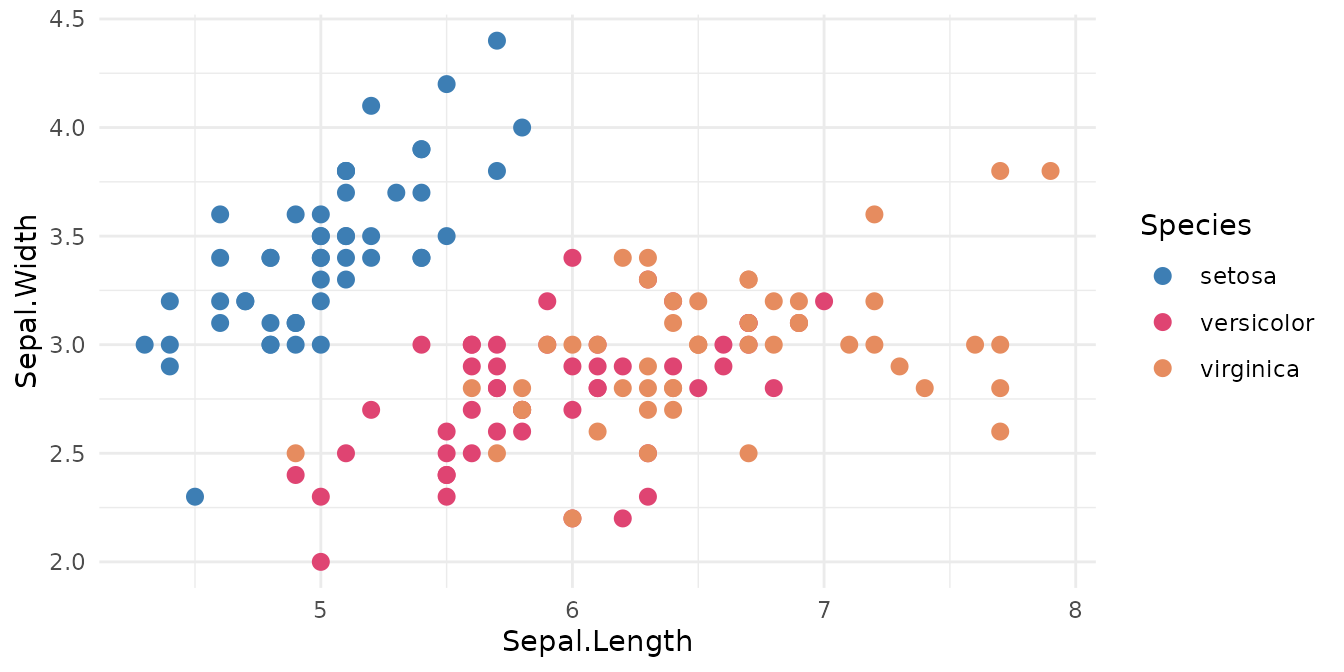
ggplot(mpg, aes(class, fill = drv)) +
  geom_bar() +
  scale_fill_japanesecolors("avantgarde_tri_06") +
  theme_minimal()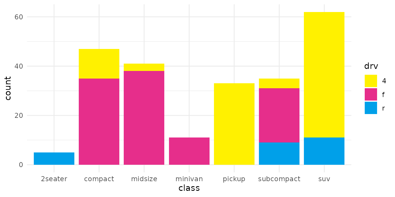
All three take reverse, na.value, and
anything else scale_*_manual() accepts:
ggplot(iris, aes(Sepal.Length, Sepal.Width, colour = Species)) +
  geom_point(size = 2.5) +
  scale_colour_japanesecolors("retro_tri_02", reverse = TRUE, name = "Iris species") +
  theme_minimal()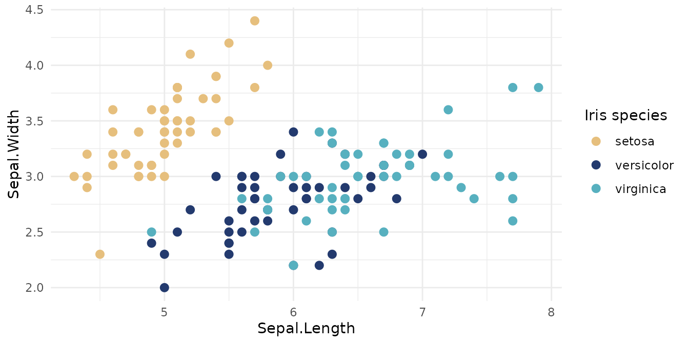
Being plain vectors, they also work with
scale_colour_manual(), which lets you pin colours to
specific categories:
cols <- setNames(kawaii_tri_07, levels(iris$Species))

ggplot(iris, aes(Sepal.Length, Sepal.Width, colour = Species)) +
  geom_point(size = 2.5) +
  scale_colour_manual(values = cols) +
  theme_minimal()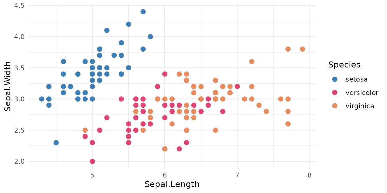
For packages that expect a palette function of
n, use japanesecolors_pal():
pal <- japanesecolors_pal("minimalism_multi_05")
pal(3)
#> [1] "#5BAE7F" "#B1C06B" "#EDDE7B"
Which palettes suit a chart
These are design palettes, so most were never meant to encode
categories. dataviz_friendly screens for the two things
that decide it: whether the colours survive colour-vision deficiency,
and whether they are far enough apart to read as different at a
glance.
nrow(palettes(dataviz_friendly = TRUE))
#> [1] 65

palettes(dataviz_friendly = TRUE, n = 4)[, c("id", "min_delta_e", "min_delta_e_cvd")]
#>                   id min_delta_e min_delta_e_cvd
#> 1      retro_four_02        22.6            11.4
#> 2      retro_four_04        26.8            13.2
#> 3      retro_four_06        24.0            12.1
#> 4      retro_four_07        24.9            15.4
#> 5      retro_four_11        23.4            10.1
#> 6 minimalism_four_06        25.0            11.4
#> 7     kawaii_four_01        30.8            10.3
#> 8 avantgarde_four_01        33.9            13.2
#> 9 avantgarde_four_02        46.0            27.4
show_palette("avantgarde_four_02")
min_delta_e is the closest pair in normal vision and
min_delta_e_cvd the closest under the worst of simulated
deuteranopia, protanopia and tritanopia, both as CIEDE2000 distances.
They ship with every palette, so you can set a different bar than the
default.
Transcription status
Colour values were read by hand from printed RGB labels. Readings that were not reliably legible are recorded as provisional:
palettes_needing_review()[1:3, c("palette_id", "order", "hex")]
#>    palette_id order     hex
#> 1 retro_bi_13     1 #F4C03A
#> 2 retro_bi_14     1 #3071B9
#> 3 retro_bi_14     2 #E34950
They are exported like any other, and palettes()
includes them by default with status == "review". For fully
transcribed values only:
See the package README for where the data came from.